Bag File Plotting

In the first part, we will learn how to record data to a bag file (Record a Bag File) and how access this data for plotting and further evaluation (Extract Data From a Bag File).

In the second part, we will go through a suggested workflow to plot this data in a thesis-/paper-/report-ready format that makes the reviewer happy, because we provide him with beautiful vector graphics with appropriate font sizes, scaling and line thicknesses. This way, the reader is not distracted and can appreciate the relevant information of the plot.

Record a Bag File

Prerequisites

To follow along this tutorial with an identical setup, we suggest the launch setup from assignment 1:

$ ros2 launch fav simulation.launch.py vehicle_name:=bluerov00

and our control setup

$ ros2 launch depth_control depth_control_full.launch.py vehicle_name:=bluerov00 use_sim_time:=true

In general, you could also use any other setup and adapt the instructions where needed.

Recording the Bag

We use the command line tool ros2 bag record for recording bag files. See the official docs for more details.

In general, we have to specify which topics we want to record and the name of the output file. The latter is optional and if not specified, the name will be the current date and time. We encourage you to choose a meainingful file name. This way it is easier to manage your bag files later on.

We can either choose each topic name manually. If we are interested in many topics, this might be not that convenient. Alternatively, we can instruct ros2 bag record to record all topics. This is very convenient, but might lead to unecessary large bag files, which might get us into trouble. Furthermore, subscribing to all topics might even overload the network capacity and negatively impact our system.

Note

Choose the topics to record wisely.

As a sensible suggestion, we provide you with the following snippet. Before you enter the command we recommend to go to the target directoy where you want the file to be saved

$ ros2 bag record -a --exclude-regex '(.*)camera(.*)' -o my_bag_file

Let’s have a detailed look at the command

-a

Record everything. This way we do not have to specify individual topics.

–exclude-regex '(.*)camera(.*)'

Exclude certain topics. We can either write them out directly or we can use regular expressions. The '(.*)camera(.*)' matches any topic name containing the substring camera. This way we avoid the most likely unncessary subscription of camera related topics, including camera images.

The command will print the topics it subscribes to on the screen. This way we can already check if the topics we wanted to subscribe are actually recorded.

$ ros2 bag record -a --exclude-regex '(.*)camera(.*)' -o my_bag_file

[INFO] [1699443379.136203027] [rosbag2_recorder]: Press SPACE for pausing/resuming
[INFO] [1699443379.149421111] [rosbag2_recorder]: Listening for topics...
[INFO] [1699443379.149427346] [rosbag2_recorder]: Event publisher thread: Starting
[INFO] [1699443379.165404721] [rosbag2_recorder]: Subscribed to topic '/tf_static'
[INFO] [1699443379.167117074] [rosbag2_recorder]: Subscribed to topic '/tf'
[INFO] [1699443379.172027901] [rosbag2_recorder]: Subscribed to topic '/parameter_events'
[INFO] [1699443379.174665871] [rosbag2_recorder]: Subscribed to topic '/events/write_split'
[INFO] [1699443379.179409041] [rosbag2_recorder]: Subscribed to topic '/rosout'
[INFO] [1699443379.186010634] [rosbag2_recorder]: Subscribed to topic '/bluerov00/odometry'
[INFO] [1699443379.186489321] [rosbag2_recorder]: Recording...
[INFO] [1699443379.837613418] [rosbag2_recorder]: Subscribed to topic '/bluerov00/thruster_command'
[INFO] [1699443379.953955551] [rosbag2_recorder]: Subscribed to topic '/bluerov00/thrusts'
[INFO] [1699443379.962161809] [rosbag2_recorder]: Subscribed to topic '/clock'
[INFO] [1699443379.971717827] [rosbag2_recorder]: Subscribed to topic '/bluerov00/pressure'
[INFO] [1699443379.978513537] [rosbag2_recorder]: Subscribed to topic '/bluerov00/ground_truth/pose'
[INFO] [1699443379.981857609] [rosbag2_recorder]: Subscribed to topic '/bluerov00/ground_truth/odometry'
[INFO] [1699443379.988602954] [rosbag2_recorder]: Subscribed to topic '/bluerov00/imu'
[INFO] [1699443379.991957938] [rosbag2_recorder]: Subscribed to topic '/bluerov00/esc_rpm'
[INFO] [1699443379.997513827] [rosbag2_recorder]: Subscribed to topic '/bluerov00/angular_velocity'
[INFO] [1699443380.002118454] [rosbag2_recorder]: Subscribed to topic '/bluerov00/acceleration'
[INFO] [1699443380.255532039] [rosbag2_recorder]: Subscribed to topic '/bluerov00/thrust_setpoint'
[INFO] [1699443380.264418114] [rosbag2_recorder]: Subscribed to topic '/bluerov00/depth_setpoint'
[INFO] [1699443380.379486377] [rosbag2_recorder]: Subscribed to topic '/bluerov00/depth'
[INFO] [1699443444.550188742] [rosbag2_cpp]: Writing remaining messages from cache to the bag. It may take a while
[INFO] [1699443444.577895499] [rosbag2_recorder]: Event publisher thread: Exiting
[INFO] [1699443444.578708119] [rosbag2_recorder]: Recording stopped
[INFO] [1699443444.604525312] [rosbag2_recorder]: Recording stopped

Note

The recording is stopped with Ctrl + C.

Inspecting the Bag File

To see important information of the recorded bag file, we use

$ ros2 bag info my_bag_file/

Note the Count entry at the end of the topic lines. This way you can verify that messages have been recorded.

$ ros2 bag info my_bag_file/

Files:             my_bag_file_0.mcap
Bag size:          16.5 MiB
Storage id:        mcap
Duration:          65.352s
Start:             Nov  8 2023 11:36:19.187 (1699443379.187)
End:               Nov  8 2023 11:37:24.539 (1699443444.539)
Messages:          103159
Topic information: Topic: /bluerov00/thrust_setpoint | Type: hippo_msgs/msg/ActuatorSetpoint | Count: 5224 | Serialization Format: cdr
                   Topic: /bluerov00/depth_setpoint | Type: hippo_msgs/msg/Float64Stamped | Count: 3214 | Serialization Format: cdr
                   Topic: /bluerov00/acceleration | Type: geometry_msgs/msg/Vector3Stamped | Count: 3146 | Serialization Format: cdr
                   Topic: /bluerov00/angular_velocity | Type: hippo_msgs/msg/AngularVelocity | Count: 15730 | Serialization Format: cdr
                   Topic: /bluerov00/esc_rpm | Type: hippo_msgs/msg/EscRpms | Count: 15731 | Serialization Format: cdr
                   Topic: /clock | Type: rosgraph_msgs/msg/Clock | Count: 15738 | Serialization Format: cdr
                   Topic: /events/write_split | Type: rosbag2_interfaces/msg/WriteSplitEvent | Count: 0 | Serialization Format: cdr
                   Topic: /bluerov00/ground_truth/odometry | Type: nav_msgs/msg/Odometry | Count: 3157 | Serialization Format: cdr
                   Topic: /tf | Type: tf2_msgs/msg/TFMessage | Count: 3186 | Serialization Format: cdr
                   Topic: /bluerov00/thruster_command | Type: hippo_msgs/msg/ActuatorControls | Count: 5467 | Serialization Format: cdr
                   Topic: /bluerov00/odometry | Type: nav_msgs/msg/Odometry | Count: 3186 | Serialization Format: cdr
                   Topic: /parameter_events | Type: rcl_interfaces/msg/ParameterEvent | Count: 0 | Serialization Format: cdr
                   Topic: /bluerov00/pressure | Type: sensor_msgs/msg/FluidPressure | Count: 5246 | Serialization Format: cdr
                   Topic: /bluerov00/thrusts | Type: hippo_msgs/msg/ThrusterForces | Count: 15740 | Serialization Format: cdr
                   Topic: /tf_static | Type: tf2_msgs/msg/TFMessage | Count: 1 | Serialization Format: cdr
                   Topic: /bluerov00/ground_truth/pose | Type: geometry_msgs/msg/PoseStamped | Count: 3157 | Serialization Format: cdr
                   Topic: /bluerov00/depth | Type: hippo_msgs/msg/DepthStamped | Count: 5213 | Serialization Format: cdr
                   Topic: /rosout | Type: rcl_interfaces/msg/Log | Count: 23 | Serialization Format: cdr
                   Topic: /bluerov00/imu | Type: sensor_msgs/msg/Imu | Count: 0 | Serialization Format: cdr

Note

Nothing is more frustrating than recording bag files while having some great experiment-time, but when we get home, we realize that the bag file is empty and no data has been recorded! Make sure, this is not happening to you.

Often it is quite useful to have a look on the recorded data even during the lab session. Luckily, this is rather easy to accomplish with plotjuggler as described here.

Extract Data From a Bag File

“Dude, we already have such a nice plot of our bag file data in plotjuggler, what else could we possibly want?”
True that, but a few aspects to motivate this section include but are not limited to

• the data we record is not the data we want to plot (let’s say we want to display the distance between to robots but the bag file only contains the position for both of the).

• we want to create a plot based on multiple subequent runs of the same experiment and overlay/combine them.

• we need to annotate our plot or highlight some sections

• we want our plot to of visually sufficient quality to support the information we would like to present sufficiently well (lines that are too thin, axis labels that are hardly readable, etc. all distract from the information that should be conveyed by the plot).

Workflow

We suggest the following workflow.

1. Read the bag file from within a python program.

2. Do the required data processing in python with numpy. numpy is the de-facto standard library for number crunching in python.

3. Preview the plots directly in python with matplotlib. matplotlib is the de-facto standard plotting library in python. With its submodule pyplot it should feel very familiar to the way we would plot in Matlab.

4. Export the data we want to finally plot as .csv file.

5. Look forward in joyful anticipation of the creation of the final plot in LaTex.

Load the Bag File

Note

We will use the simulation setup based on assignment 1 for demonstration purposes. The general workflow should be understandable without having done this assignment and can be easily adapted for other scenarios.

We write a python program and use the rosbag2_py modue to read the bag file.

We want to create the following directory structure:

~/fav/bag_evaluation
├── main.py
├── my_bag_file
│   ├── metadata.yaml
│   └── my_bag_file_0.mcap
└── reader.py

Note

We can create this directory and the main.py and reader.py directly inside VSCode! Remember, that you need to make them executable. The my_bag_file directory is the bag file directory created via ros2 bag record.

Create a Preview Plot

We copy-paste the following code into reader.py

reader.py

import rosbag2_py
from rclpy.serialization import deserialize_message
from rosidl_runtime_py.utilities import get_message


class Reader():

    def __init__(self, bag_file: str):
        self.bag_file = bag_file

    def _read_topic(self, selected_topic: str):
        reader = rosbag2_py.SequentialReader()
        reader.open(
            rosbag2_py.StorageOptions(uri=self.bag_file, storage_id="mcap"),
            rosbag2_py.ConverterOptions(input_serialization_format="cdr",
                                        output_serialization_format="cdr"),
        )
        topic_types = reader.get_all_topics_and_types()

        def typename(topic_name):
            for topic_type in topic_types:
                if topic_type.name == topic_name:
                    return topic_type.type
            raise ValueError(f'topic {topic_name} not in bag')

        while reader.has_next():
            topic, data, timestamp = reader.read_next()
            if topic != selected_topic:
                continue
            msg_type = get_message(typename(topic))
            msg = deserialize_message(data, msg_type)
            yield topic, msg, timestamp
        del reader

    def get_data(self, topic: str):
        return [[x[1], x[2]] for x in self._read_topic(topic)]

We do not care for the details of the reader implementation for now. It simply provides us with the functionality to read data from the bag file.

We do the same for the content of main.py with the following code:

main.py

#!/usr/bin/env python3

from reader import Reader
import matplotlib.pyplot as plt
import numpy as np


def plot_depth_vs_setpoint(reader: Reader):
    setpoint_data = reader.get_data('/bluerov00/depth_setpoint')
    n_messages = len(setpoint_data)
    depth_setpoints = np.zeros([n_messages])
    t_setpoints = np.zeros([n_messages])

    i = 0
    for msg, time_received in setpoint_data:
        depth_setpoints[i] = msg.data
        t_setpoints[i] = time_received * 1e-9
        i += 1

    depth_data = reader.get_data('/bluerov00/depth')
    n_messages = len(depth_data)
    depth = np.zeros([n_messages])
    t_depth = np.zeros([n_messages])

    i = 0
    for msg, time_received in depth_data:
        depth[i] = msg.depth
        t_depth[i] = time_received * 1e-9
        i += 1

    plt.figure()
    plt.plot(t_setpoints, depth_setpoints, label='Depth Setpoint')
    plt.plot(t_depth, depth, label='Current Depth')
    plt.legend()
    plt.show()


def main():
    reader = Reader('my_bag_file')
    plot_depth_vs_setpoint(reader)


if __name__ == '__main__':
    main()

Not to be Captain Obvious again, but don’t forget to update the argument in reader = Reader('my_bag_file') to your bag’s actual name. 👀

In a terminal (an integrated one of VSCode or open a new one with Ctrl + Alt + T) we make sure we are in the same directory as the main.py file

$ cd ~/fav/bag_evaluation

and run the main.py script:

$ python3 main.py

Which yields the following plot (or a similar one):

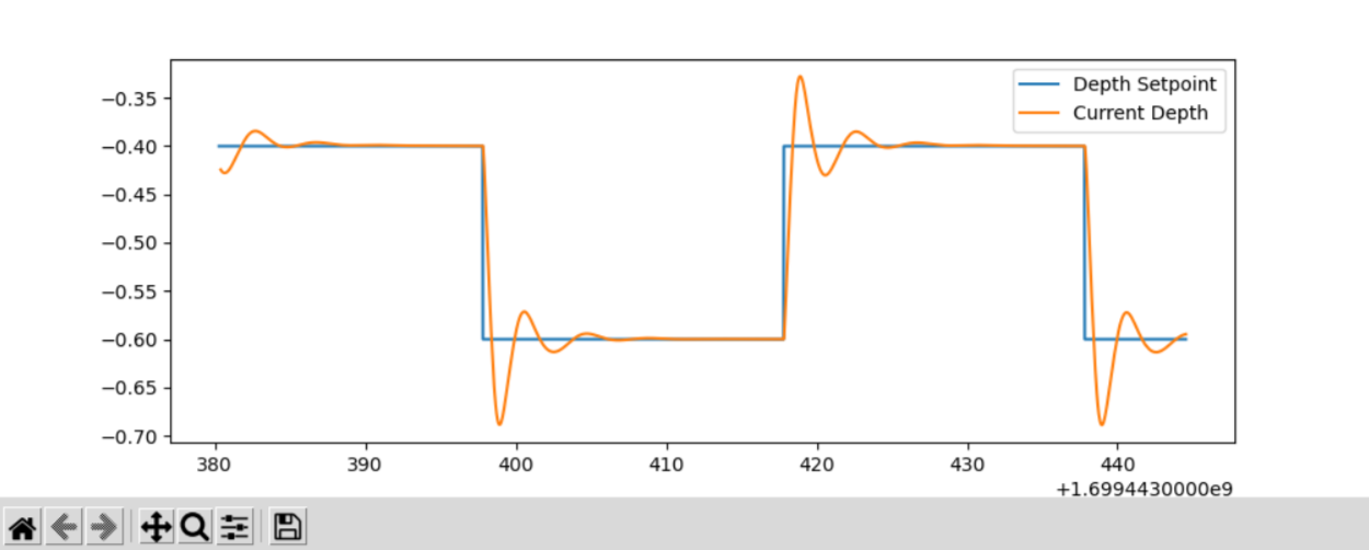
Congrats, our first manually created plot from extracted bag file data! 🥳

Don’t see a plot?

Firstly, we recommend (if not already done before) to inspect the bag file, making sure, your desired topics have been recorded at all:

$ ros2 bag info my_bag_file/

Well, to check if there is anything wrong with our bag file, we can check the data by simply exchanging the main.py content to the following snippet:

main.py

#!/usr/bin/env python3

from reader import Reader

def main():
    reader = Reader('my_bag_file')
    data = reader.get_data('/bluerov00/depth_setpoint')

    for (msg, time_received) in data:
        print(f'Message: {msg}\ntime_received: {time_received}')


if __name__ == '__main__':
    main()

If you execute main.py now, you should get a list of messages printed to the screen, each one representing recorded data at a specific time:

$ python3 main.py
...
Message: hippo_msgs.msg.Float64Stamped(header=std_msgs.msg.Header(stamp=builtin_interfaces.msg.Time(sec=1699443444, nanosec=495445714), frame_id=''), data=-0.6)
time_received: 1699443444495922280
Message: hippo_msgs.msg.Float64Stamped(header=std_msgs.msg.Header(stamp=builtin_interfaces.msg.Time(sec=1699443444, nanosec=515611158), frame_id=''), data=-0.6)
time_received: 1699443444516101056
Message: hippo_msgs.msg.Float64Stamped(header=std_msgs.msg.Header(stamp=builtin_interfaces.msg.Time(sec=1699443444, nanosec=535362893), frame_id=''), data=-0.6)
time_received: 1699443444536112988

This is one way, you could check for discrepancies.

Note

Old habits die hard. For the sake of simplicity we did not label the axes. We wouldn’t go so far to call it best-practice. Even if we only strive for barely-good-enough, we should add axes labels to any plot we create. So better do not get used to omitting the labels.

Crop the Data to a meaningful Time-Span

Lets have the plot begin 5 seconds before a setpoint change and end after the second setpoint change, so that we end up with a plot containing upward and downward changes of the setpoint.

A quick way to do this is by hovering with the cursor over the plot to see at which point in time the first setpoint change happens. When we do this, the coordinates are shown in the lower right corner of the plotting window.

For this very plot the first setpoint change happens at 1699443397.7s. Since we want our plot to start with \(t_0=0\,\mathrm{s}\) five seconds earlier, we subtract the corresponding time. The required code changes are highlighted below

main.py

#!/usr/bin/env python3

from reader import Reader
import matplotlib.pyplot as plt
import numpy as np


def plot_depth_vs_setpoint(reader: Reader):
    t_offset = 1699443392.7
    setpoint_data = reader.get_data('/bluerov00/depth_setpoint')
    n_messages = len(setpoint_data)
    depth_setpoints = np.zeros([n_messages])
    t_setpoints = np.zeros([n_messages])

    i = 0
    for msg, time_received in setpoint_data:
        depth_setpoints[i] = msg.data
        t_setpoints[i] = time_received * 1e-9
        i += 1
    t_setpoints -= t_offset

    depth_data = reader.get_data('/bluerov00/depth')
    n_messages = len(depth_data)
    depth = np.zeros([n_messages])
    t_depth = np.zeros([n_messages])

    i = 0
    for msg, time_received in depth_data:
        depth[i] = msg.depth
        t_depth[i] = time_received * 1e-9
        i += 1
    t_depth -= t_offset

    plt.figure()
    plt.plot(t_setpoints, depth_setpoints, label='Depth Setpoint')
    plt.plot(t_depth, depth, label='Current Depth')
    plt.legend()
    plt.show()


def main():
    reader = Reader('my_bag_file')
    plot_depth_vs_setpoint(reader)


if __name__ == '__main__':
    main()

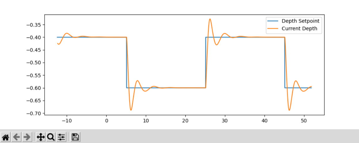
Now the plot should look like this:

Note

If you want to plot further topics, ensure that you also include the offset for each additional data series

For cropping the data to the area of our interest, we provide you with a cropping function that we add to main.py.

The enhanced main.py looks like

main.py

#!/usr/bin/env python3

from reader import Reader
import matplotlib.pyplot as plt
import numpy as np


def crop_data(data, time, t0, t1):
    tmp = np.abs(time - t0)
    a = tmp.argmin()
    tmp = np.abs(time - t1)
    b = tmp.argmin()
    return data[a:b], time[a:b]


def plot_depth_vs_setpoint(reader: Reader):
    t_offset = 1699443392.7
    t_start = 0.0
    t_end = 45.0
    setpoint_data = reader.get_data('/bluerov00/depth_setpoint')
    n_messages = len(setpoint_data)
    depth_setpoints = np.zeros([n_messages])
    t_setpoints = np.zeros([n_messages])

    i = 0
    for msg, time_received in setpoint_data:
        depth_setpoints[i] = msg.data
        t_setpoints[i] = time_received * 1e-9
        i += 1
    t_setpoints -= t_offset
    depth_setpoints, t_setpoints = crop_data(depth_setpoints, t_setpoints,
                                             t_start, t_end)

    depth_data = reader.get_data('/bluerov00/depth')
    n_messages = len(depth_data)
    depth = np.zeros([n_messages])
    t_depth = np.zeros([n_messages])

    i = 0
    for msg, time_received in depth_data:
        depth[i] = msg.depth
        t_depth[i] = time_received * 1e-9
        i += 1
    t_depth -= t_offset
    depth, t_depth = crop_data(depth, t_depth, t_start, t_end)

    plt.figure()
    plt.plot(t_setpoints, depth_setpoints, label='Depth Setpoint')
    plt.plot(t_depth, depth, label='Current Depth')
    plt.legend()
    plt.show()


def main():
    reader = Reader('my_bag_file')
    plot_depth_vs_setpoint(reader)


if __name__ == '__main__':
    main()

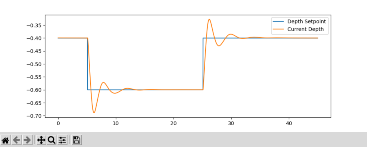
which in our case produces the following plot when we run it

Export the Plot Data

This looks almost like we finished the plotting. But now we have to export this plot/data into a csv file that us used to create the very same plot directly in LaTex.

We create the additional directory export in our bag_evaluation directory (via the following command or directly in VSCode)

$ mkdir ~/fav/bag_evaluation/export

Check that your directory structure looks similar to

~/fav/bag_evaluation
├── export
├── main.py
├── my_bag_file
│   ├── metadata.yaml
│   └── my_bag_file_0.mcap
└── reader.py

Writing the csv can be implemented real quick and can be seen at the highlighted lines below

main.py

#!/usr/bin/env python3

from reader import Reader
import matplotlib.pyplot as plt
import numpy as np


def crop_data(data, time, t0, t1):
    tmp = np.abs(time - t0)
    a = tmp.argmin()
    tmp = np.abs(time - t1)
    b = tmp.argmin()
    return data[a:b], time[a:b]


def plot_depth_vs_setpoint(reader: Reader):
    t_offset = 1699443392.7
    t_start = 0.0
    t_end = 45.0
    setpoint_data = reader.get_data('/bluerov00/depth_setpoint')
    n_messages = len(setpoint_data)
    depth_setpoints = np.zeros([n_messages])
    t_setpoints = np.zeros([n_messages])

    i = 0
    for msg, time_received in setpoint_data:
        depth_setpoints[i] = msg.data
        t_setpoints[i] = time_received * 1e-9
        i += 1
    t_setpoints -= t_offset
    depth_setpoints, t_setpoints = crop_data(depth_setpoints, t_setpoints,
                                             t_start, t_end)
    data = np.hstack(
        [t_setpoints.reshape(-1, 1),
         depth_setpoints.reshape(-1, 1)])
    np.savetxt('export/depth_setpoint.csv',
                data,
                delimiter=',',
                header='t, depth_setpoint',
                comments='')

    depth_data = reader.get_data('/bluerov00/depth')
    n_messages = len(depth_data)
    depth = np.zeros([n_messages])
    t_depth = np.zeros([n_messages])

    i = 0
    for msg, time_received in depth_data:
        depth[i] = msg.depth
        t_depth[i] = time_received * 1e-9
        i += 1
    t_depth -= t_offset
    depth, t_depth = crop_data(depth, t_depth, t_start, t_end)

    data = np.hstack([t_depth.reshape(-1, 1), depth.reshape(-1, 1)])
    np.savetxt('export/depth.csv',
                data,
                delimiter=',',
                header='t, depth',
                comments='')

    plt.figure()
    plt.plot(t_setpoints, depth_setpoints, label='Depth Setpoint')
    plt.plot(t_depth, depth, label='Current Depth')
    plt.legend()
    plt.show()


def main():
    reader = Reader('my_bag_file')
    plot_depth_vs_setpoint(reader)


if __name__ == '__main__':
    main()

After running python3 main.py there should be the correspond csv files in the export directory. You can directly check this in VSCode or via the command line

$ ls ~/fav/bag_evaluation/export
depth.csv  depth_setpoint.csv

Create Beautiful Plots in LaTex

We will share/have shared a LaTex template via Overleaf with you. There is an example for plotting the data already implemented.

We recommend to create a separate tex file for each plot inside the /plots/ directory. Thus, the file structure of the LaTex project would look like

/plots
├── data
│   ├── depth_setpoint.csv
│   └── depth.csv
└── depth_plot.tex

The data directory contains the csv files we exported in the previous section. The actual plotting is done in plots/depth_plot.tex with pgfplots in a tikz environment. Hence, both of these are useful keywords when using your favourite search engine how to accomplish certain things when it comes to plotting data.

For the sake of completeness, we present the content of depth_plot.tex and a typical way to include this plot in a figure.

depth_plot.tex

\begin{tikzpicture}
    \begin{axis} [
        % scale the plot relative to available space
        width=\linewidth,
        height=0.4\linewidth,
        % we know our plot starts at t=0 and has a duration of 45s.
        xmin=0,
        xmax=45,
        ymin=-0.7,
        ymax=-0.3,
        % a grid is often a valuable visual aid
        grid=both,
        % always label the axes!
        xlabel={Time (s)},
        ylabel={Depth (m)},
        % if not unambiguous, add a legend to the plot.
        % otherwise the viewer cannot know which line corresponds to what.
        legend entries = {Setpoint, Depth},
        % the default position would be top right.
        % to not have the legend covering a part of our plot, we move
        % it to the bottom right corner.
        legend style={at={(1, 0)}, anchor=south east, xshift=-2mm, yshift=2mm},
    ]

    % usually, anything smaller than thick lines is too small.
    \addplot+[thick, dashed, black]
        % we choose the data for x and y by name specified in the
        % first line of our csv file.
        table [x=t, y=depth_setpoint, col sep=comma]
        % specify the data file to get the data from
        {plots/data/depth_setpoint.csv};

    \addplot+[thick, mumred]
        table [x=t, y=depth, col sep=comma]
        {plots/data/depth.csv};
    \end{axis}
\end{tikzpicture}

We then include this plot inside a figure environment in our main.tex file.

main.tex

% ... some content before
\begin{figure}
    \centering
    \input{plots/depth_plot}
    \caption{Add a sufficiently descriptive caption here!}
    \label{fig:depth-plot}
\end{figure}
% ... some content after

For more detailed plot configurations use the publicly available resources. There are so many options to configure a plot which would definitely go beyond the scope of this tutorial.